In this post I will share yet another tool from my PM Toolbox: A simple method any Software Project Manager can use for predicting the likelihood of project completion, based on a model for defect prediction. This tool only scratches the surface of real software engineering defect management, but has nevertheless proved useful in my experience of managing a large software stack. For instance, this tool was borne from my direct experiences as a Development Owner for a large Software Stack for STB Middleware that comprised of more than eighty (80) software components, where each component was independently owned and subject to specific defect & software code quality requirements. I needed a tool to help me predict when the software was likely to be ready for launch based on the health of the open defects; as well as use it as evidence to motivate to senior management to implement recovery scenarios. It was quite useful (and relatively accurate within acceptable tolerances) as it offered perspective of a reality that more often than not, people underestimate the work required to get defects under control, the need for predicting project completion dates based of defect resolution rates, depending on the maturity of the team is often also misunderstood.
I created the first instance of this tool back in 2008/2009, the first public version was shared in this post on Effective Defect & Quality Management. Since then, I've upgraded the tool to be more generic, and also significantly cut down on the number of software components. I still use the tool in my ongoing projects, and have recently convinced senior management in my current project to pay heed to defect predictions.
Why the need for Defect Predictions / Metrics?
This might be a no-brainer for most people who are seasoned practitioners of software product development and are keen supporters of sound software engineering principles, but you'll be surprised how often people ask this question, especially in young development teams who might have very good skills in coding, but lack appreciation for software engineering management. A software project manager used to applying best practices might find himself/herself butting heads with development managers about implementing quality improvements that should be well accepted practices instead of wasting time debating whether there's a need for it or not!
I've had this challenge recently where not only the internal development teams, but also the vendors involved are pretty new to the whole Set-Top-Box (STB) Software Product space, but have exceptional programmers writing code. I would rate their coding skills around 7/10 but their software engineering skills around a 4/10.
There is a big difference between being a great coder and a great software engineer IMHO. Engineering relies on strong analysis, measurement and feedback loops in engineering management to continuously improve on the quality of your deliverable.
When a young start-up development team embarks on a project, all they can think about is getting to code complete, and when the Project Manager starts asking some interesting questions about code quality, defect management, and predicting defect resolution rates based on productivity history, then almost naturally, this young development team will flout the "Agile versus Waterfall" heavy handed project management styles which really makes a weak defense!
Alas, applying software engineering best practices has really nothing to do with whether you're doing Agile or not. In fact, Agile is quite strong on quality control and measuring productivity.
There is a huge body of knowledge on the subject of Software Quality Management & Measurement, that development teams should take as a given and not argue with! I've written in the past about The Importance of Defect Metrics that I won't repeat here. For more info read this post, as well as lookup the popular cited-references in the side bar.
A DTV project is a naturally software-intensive system, and as such, a key measurement of software systems is the latent state of bugs or defects.
Taking a few words out of Steve McConnell's Software Project Survival Guide: How to be Sure Your First Important Project isn't Your Last (Pro -- Best Practices)
At the most basic level, defect counts give you a quantitative handle on how much work the project team has to do before it can release the software. By comparing the number of defects resolved each week, you can determine how close the project is to completion. If the number of new defects in a particular week exceeds the number of defects resolved that week, the project still has miles to go...

If the project’s quality level is under control and the project is making progress toward completion, the number of open defects should generally trend downward after the middle of the project, and then remain low. The point at which the “fixed” defects line crosses the “open” defects line is psychologically significant because it indicates that defects are being corrected faster than they are being found. If the project’s quality level is out of control and the project is thrashing (not making any real progress toward completion), you might see a steadily increasing number of open defects. This suggests that steps need to be taken to improve the quality of the existing designs and code before adding more new functionality…
Recap Set-Top-Box Context
Set-Top-Box projects that have not evolved to implementing Agile in its true form, i.e. to continuously deliver fully functional software stack every iteration with little or no regression, tend to instead focus on reaching the first major milestone of Feature Complete with open defects, then embark on a Stabilisation/Test phase where the main focus is on burning down the open defects to reach a Launch Candidate build. The typical scenario is shown here:
Development Stage -> Feature Complete -> Launch Candidate 1 -> ... -> Launch Candidate N -> Deploy
At each stage there will be a backlog of open defects that are prioritized on a daily basis, with a focus on priority for launch. I've written about setting specific and clear targets for milestones as well as defining clear defect criteria. I've also written about the general Release Campaign model for releases leading up to Launch. You will also find my model for planning STB projects useful background information, as each stage needs to meet some acceptance criteria, of which Open Defects is one such condition.
So the focus for defect predictions will be measuring progress towards reaching some targets for the milestones. The focus usually is on Showstoppers (Priority Zeros "P0s") & Majors (Priority Ones "P1s"). Generally the project will set an acceptable target for the allowed P0s & P1s at Launch. I support the view of having zero P0s at launch, but in reality this is hard to achieve, and often the PayTV operator, depending on its respect for quality, will launch a product with a small number of open P0s, a fairly large number of open P1s, targeting a maintenance release post-launch, within 3 months to clear out as much of the remaining defects as possible.
Again, this is old-school management in my view - I believe it is possible to deliver value with incremental iterations without compromising quality, such that the need for a separate "Stabilisation & Test" phase disappears almost entirely. It can be done, but requires a significant change in mindset, and a massive focus on engineering quality in all development/integration processes from the start of a project...
Walkthrough of My Defect Prediction Model
A Defect prediction tool must track specific targets - a typical DTV project will maintain specific targets for all the software components in the end-to-end-value chain. Typically, the project follows a staged process as described in earlier, which are broadly accepted as:
Feature Complete (Dev Complete) -> Functionally Complete (FC) -> Launch Candidate 1 -> Launch Candidate 2 -> Launch Candidate 3 -> Launch Build -> Deployment Build
At each stage, we will have set targets to reach in terms of allowable open P0/Showstopper & P1/Major defects, with decreasing numbers reaching Zero for P0s/Showstoppers to Lower Tens for P1s/Majors. In reality however, most DTV projects go-live with outstanding P0s/Showstoppers, but these are generally not obvious defects and deemed acceptable by the business to risk the product launch with those defects still not fixed - that's just the way these projects go!
What typically happens with these projects, especially STB projects, is that much of the formal testing is left towards the closing stages of the development & integration phase. For example, certification tests like HDMI, Dolby Digital, CE & other mandatory tests required from a consumer electronics product can only be done when the required software components are reasonably stable. The PayTV Operator also tends to get involved with formal QA processes (CE-QA / ATP) toward the end, as well as, the Field Trial process (where the product is subjected to real-world home testing by real users) is also started late in the project. Of course the project management team will have mitigated this by testing early and initiating Engineering Field trials early -- but it is still expected that these additional QA stages serve as injection points and add to the overall Defect Pool that must be managed.
Below is a picture of how I recently described the theory to my colleagues including some senior managers:
The above picture illustrates the trend of defects through the life cycle of a project. The Red curve shows the Submitted Defects, whilst the Blue curve shows the Closed Defects respectively. Initially, during the early stages of the the project, the development team will take a while to start closing down defects, and for some time there will remain more defects being submitted than defects closed. At some point, the submitted defects will peak (as shown by "PEAK" in the first graph), and the Closed curve should overtake the Submitted Curve. As above, when this happens, this is the general watershed moment. At certain stages such as ATP/CEQA, and Field Trials, expect a spike in submitted defects (as shown by red dotted peaks), but expect overall that the Submitted curve decreases over time, aiming to reach zero at some point. The second graph zooms in on weekly comparison of Submit Rate V Close Rate. As long as the Close Rate is less than the Submit Rate, that component has a while to go yet. If there is a big gap as shown in the shaded "BAD" area, this means the team has still a steep climb ahead. As soon as the watershed moment is reach, things start to look good, and assuming this wasn't a once-off occurrence, and the trend is on the increase, then the team should aim to widen the gap between Closed & Submitter, as shown by "INC GAP = GOOD" meaning that this component has reach a status of having good control of its defects...
A Defect Modelling tool therefore must take into account the following:
The Model simply is a function of Submission Rate versus Closure Rate. The unit of measure is weekly. I've chosen weekly time samples out of my experience with STB projects that once the Feature/Functionally Complete stage is reached, we generally are working in bug-fixing & stabilisation mode where we produce weekly releases. This is regardless of whether your sprint cycles are two weeks or six weeks in duration - it is expected that teams are using the defect tracking systems on a daily basis where we can track progress of defects daily, instead of the end of a cycle.
Weekly snapshots gives enough granularity for management to track progress in a more controlled manner, as it is neither too long nor too short. Doing it daily is just plain excessive, whilst doing it monthly is likely to hide patterns (problem areas) that will go unnoticed until it's too late. Weekly snapshots in my experience provides just the right balance, giving management enough of an insiders-view to instigate discussions around interventions, etc.
Submission Rate is the number of defects submitted or discovered over a week. This is the number of new defects incoming.
Closure Rate is the number of defects marked as closed by your Development/QA team. You have to be really careful with your defect tracking tool here, since defects will have certain number of states, that mean different things to different people. For the model, we base the information on Actual status - meaning that defects are "closed" when they in a state of "Verified, Closed, Rejected, Duplicate". Any defect not in either of these states are considered "Open". This includes defects waiting to be tested & verified, even though the component vendor might have marked the defect as "Resolved, Ready for Test, Awaiting Verification", etc.
Formula for Open Defects is simple:
Num. defects Predicted Open Next Week = Number Currently Open + Submit Rate - Close Rate
where
Submit Rate = Average number of defects submitted per week
Close Rate = Average number of defects closed per week
Average = Moving Average over a number of weeks going back as far as realistically possible into past history
Predicting the time to close defects to reach your target
What management are interested in, is in a rough approximation of the likelihood a component team will reach its defect targets. We first start with the current Open Defect Count and the current rolling average of Submit Rate & Closure Rate. We can tell immediately the project is never ending, i.e. will not reach its targets if the Submit Rate is currently larger than the Close Rate - i.e. we are currently raising more defects than we are currently closing - you will be more or less constant at the current open number of defects. This is illustrated in the following curve:

In this example, the Submit Rate is already larger than the Closure Rate, hence expect no end in sight!
What you want to see is a steady decline in Submit Rate, or a steady increase in Closure Rate. Now, in my own experience I prefer to assume the former scenario rather than the latter. This is because at a certain point in the project, especially past the FC stage, the rate of submissions or new defects should start to decrease and reach a plateau, i.e. start flattening out because the quality of the build should ideally improve over time.
Closure rate on the other hand is limited by forces of reality - i.e. the performance and productivity of your development team. If the team are already operating at peak capacity, then there is very little chance of the team showing vast improvements in closure rate to over take the submission rate. In the rare case that your team were perhaps cruising along and have bandwidth to inject bursts of productivity that can be sustained till the end of the project, then you can assume your closure rate will increase - although I highly doubt that!

The best course of action, the most realistic one is to safely assume your team is already max'ed out, working at full throttle, and their closure rate will remain as is - they can only work so hard. Yes, you might want to instigate bursts of overtime to get the defect counts down - but you will still max out eventually. It has been my experience to utilise overtime strategically, where needed, but seek other means of lowering the defect counts. On the other hand, your closure rate could increase if you inject more people, who are experts and require no start-up costs - this too, is very rare. So you're most likely going to end up with a model that assumes your Submission Rate will decrease over time, but your Closure Rate remains constant as shown below:

By fine-tuning the variables Submit Rate & Closure Rate, you can view different scenarios of likelihood of reaching the targets, and the reality of making such improvements. The model is not perfect, neither does it try to be a detailed scientific or mathematical simulation - it errs on the pragmatic approach that offers reasonable guidance to a project manager to use as evidence in motivating the health of the project. Note the model assumes a uniform decrease in submission rate, i.e. linear decrease week by week. This is the ideal, but in reality this might also wax and wane. There is room for correction within the model itself, to reset the submission rate or inject new defects, and thus update accordingly.
The main page of the Model is shown below:
There is just one section for User Input, the rest is automatically generated:

Here the user can select from a drop-down list, the Phase to focus on, the type of defects to filter, and a software component. The model then pulls all data from various other sheets and present both the actual trend for the rolling 9 weeks, as well as a main table & graph depicting the trend, or suggested glide path to launch based on the parameters to fine tune the Submit Rate / Closure Rate. In the above example, we're focusing on the Launch Criteria for the Middleware component, targeting combined P0/Showstoppers and P1/Major defects. We are also hoping for a 2% decrease in overall submit rate on a week by week basis. The resulting trend is then shown via a table and the glide path:
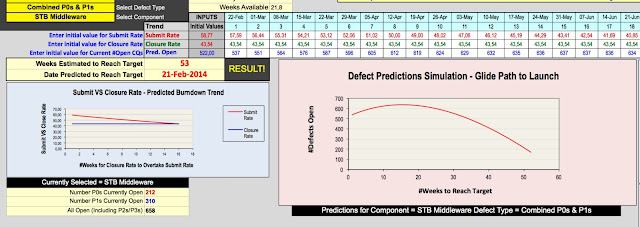
The model assumes the project has one year to launch (52 weeks) as the overall constraint - if the calculation overflows 52 weeks, the prediction engine stops and just assumes there's no hope. In the above example, even with a 2% decrease in submit rate we have no end in sight. So as a manager, you want to consider scenarios where this could change, as shown in the figure below:
 The above picture now shows that assuming a 4% improvement in Submit Rate and a 2% improvement in Closure Rate, we will reach our target criteria in 26 weeks. Still however, the current target for launch is set to 26-Jul, with only 21.8 weeks available, we overshoot by additional 5 weeks - so the probability of reaching the target is quite low.
Finally it is crucial the project defines the targets upfront, since the model depends on this:

It is also good to have some perspective over the actual trend for the past 9 weeks. I've chosen 9 weeks as this is about as realistic as it gets, because in the classic "Stabilisation/Bug-Fix" cycle, you will be iterating every week - a snapshot of the last two months is a good indicator of measuring weekly progress and a chance to gauge the performance of any management interventions:
With these trends you can assess the overall health of the particular component. For example, the above component seems to have hit a turning point recently with closing more P0s than submitted, and might possibly be starting to get a handle on the P1s as well, and overall we might just be experiencing a watershed moment, although time will tell. For this to make any sense, we need to seed and monitor for a few more weeks.
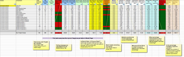
Another useful page is the "Project Predictions" tab which is basically the driver behind the model. This is where the defect history is mined, averages calculated, and based on the current number of open defects, you can tell at a glance which are the problem areas even before starting modelling different scenarios:
Feature Complete (Dev Complete) -> Functionally Complete (FC) -> Launch Candidate 1 -> Launch Candidate 2 -> Launch Candidate 3 -> Launch Build -> Deployment Build
At each stage, we will have set targets to reach in terms of allowable open P0/Showstopper & P1/Major defects, with decreasing numbers reaching Zero for P0s/Showstoppers to Lower Tens for P1s/Majors. In reality however, most DTV projects go-live with outstanding P0s/Showstoppers, but these are generally not obvious defects and deemed acceptable by the business to risk the product launch with those defects still not fixed - that's just the way these projects go!
What typically happens with these projects, especially STB projects, is that much of the formal testing is left towards the closing stages of the development & integration phase. For example, certification tests like HDMI, Dolby Digital, CE & other mandatory tests required from a consumer electronics product can only be done when the required software components are reasonably stable. The PayTV Operator also tends to get involved with formal QA processes (CE-QA / ATP) toward the end, as well as, the Field Trial process (where the product is subjected to real-world home testing by real users) is also started late in the project. Of course the project management team will have mitigated this by testing early and initiating Engineering Field trials early -- but it is still expected that these additional QA stages serve as injection points and add to the overall Defect Pool that must be managed.
Below is a picture of how I recently described the theory to my colleagues including some senior managers:
 |
| Rough sketches of concepts |
The above picture illustrates the trend of defects through the life cycle of a project. The Red curve shows the Submitted Defects, whilst the Blue curve shows the Closed Defects respectively. Initially, during the early stages of the the project, the development team will take a while to start closing down defects, and for some time there will remain more defects being submitted than defects closed. At some point, the submitted defects will peak (as shown by "PEAK" in the first graph), and the Closed curve should overtake the Submitted Curve. As above, when this happens, this is the general watershed moment. At certain stages such as ATP/CEQA, and Field Trials, expect a spike in submitted defects (as shown by red dotted peaks), but expect overall that the Submitted curve decreases over time, aiming to reach zero at some point. The second graph zooms in on weekly comparison of Submit Rate V Close Rate. As long as the Close Rate is less than the Submit Rate, that component has a while to go yet. If there is a big gap as shown in the shaded "BAD" area, this means the team has still a steep climb ahead. As soon as the watershed moment is reach, things start to look good, and assuming this wasn't a once-off occurrence, and the trend is on the increase, then the team should aim to widen the gap between Closed & Submitter, as shown by "INC GAP = GOOD" meaning that this component has reach a status of having good control of its defects...
A Defect Modelling tool therefore must take into account the following:
- Current number of Open Defects
- History to date of Defect Submission Rate (Number of defects discovered per week) & Closure Rate (Number of defects closed per week)
- Injection Points where spikes of new defects is expected to add to the defect pool
- Account for any other anomalies (e.g. decline in Closure rate, other injection points)
- Calculate forward looking predictions based on current & past behaviours
The Model simply is a function of Submission Rate versus Closure Rate. The unit of measure is weekly. I've chosen weekly time samples out of my experience with STB projects that once the Feature/Functionally Complete stage is reached, we generally are working in bug-fixing & stabilisation mode where we produce weekly releases. This is regardless of whether your sprint cycles are two weeks or six weeks in duration - it is expected that teams are using the defect tracking systems on a daily basis where we can track progress of defects daily, instead of the end of a cycle.
Weekly snapshots gives enough granularity for management to track progress in a more controlled manner, as it is neither too long nor too short. Doing it daily is just plain excessive, whilst doing it monthly is likely to hide patterns (problem areas) that will go unnoticed until it's too late. Weekly snapshots in my experience provides just the right balance, giving management enough of an insiders-view to instigate discussions around interventions, etc.
Submission Rate is the number of defects submitted or discovered over a week. This is the number of new defects incoming.
Closure Rate is the number of defects marked as closed by your Development/QA team. You have to be really careful with your defect tracking tool here, since defects will have certain number of states, that mean different things to different people. For the model, we base the information on Actual status - meaning that defects are "closed" when they in a state of "Verified, Closed, Rejected, Duplicate". Any defect not in either of these states are considered "Open". This includes defects waiting to be tested & verified, even though the component vendor might have marked the defect as "Resolved, Ready for Test, Awaiting Verification", etc.
Formula for Open Defects is simple:
Num. defects Predicted Open Next Week = Number Currently Open + Submit Rate - Close Rate
where
Submit Rate = Average number of defects submitted per week
Close Rate = Average number of defects closed per week
Average = Moving Average over a number of weeks going back as far as realistically possible into past history
Predicting the time to close defects to reach your target
What management are interested in, is in a rough approximation of the likelihood a component team will reach its defect targets. We first start with the current Open Defect Count and the current rolling average of Submit Rate & Closure Rate. We can tell immediately the project is never ending, i.e. will not reach its targets if the Submit Rate is currently larger than the Close Rate - i.e. we are currently raising more defects than we are currently closing - you will be more or less constant at the current open number of defects. This is illustrated in the following curve:
In this example, the Submit Rate is already larger than the Closure Rate, hence expect no end in sight!
What you want to see is a steady decline in Submit Rate, or a steady increase in Closure Rate. Now, in my own experience I prefer to assume the former scenario rather than the latter. This is because at a certain point in the project, especially past the FC stage, the rate of submissions or new defects should start to decrease and reach a plateau, i.e. start flattening out because the quality of the build should ideally improve over time.
Closure rate on the other hand is limited by forces of reality - i.e. the performance and productivity of your development team. If the team are already operating at peak capacity, then there is very little chance of the team showing vast improvements in closure rate to over take the submission rate. In the rare case that your team were perhaps cruising along and have bandwidth to inject bursts of productivity that can be sustained till the end of the project, then you can assume your closure rate will increase - although I highly doubt that!
The best course of action, the most realistic one is to safely assume your team is already max'ed out, working at full throttle, and their closure rate will remain as is - they can only work so hard. Yes, you might want to instigate bursts of overtime to get the defect counts down - but you will still max out eventually. It has been my experience to utilise overtime strategically, where needed, but seek other means of lowering the defect counts. On the other hand, your closure rate could increase if you inject more people, who are experts and require no start-up costs - this too, is very rare. So you're most likely going to end up with a model that assumes your Submission Rate will decrease over time, but your Closure Rate remains constant as shown below:
By fine-tuning the variables Submit Rate & Closure Rate, you can view different scenarios of likelihood of reaching the targets, and the reality of making such improvements. The model is not perfect, neither does it try to be a detailed scientific or mathematical simulation - it errs on the pragmatic approach that offers reasonable guidance to a project manager to use as evidence in motivating the health of the project. Note the model assumes a uniform decrease in submission rate, i.e. linear decrease week by week. This is the ideal, but in reality this might also wax and wane. There is room for correction within the model itself, to reset the submission rate or inject new defects, and thus update accordingly.
The main page of the Model is shown below:
 |
| Model Dashboard |
Here the user can select from a drop-down list, the Phase to focus on, the type of defects to filter, and a software component. The model then pulls all data from various other sheets and present both the actual trend for the rolling 9 weeks, as well as a main table & graph depicting the trend, or suggested glide path to launch based on the parameters to fine tune the Submit Rate / Closure Rate. In the above example, we're focusing on the Launch Criteria for the Middleware component, targeting combined P0/Showstoppers and P1/Major defects. We are also hoping for a 2% decrease in overall submit rate on a week by week basis. The resulting trend is then shown via a table and the glide path:
The model assumes the project has one year to launch (52 weeks) as the overall constraint - if the calculation overflows 52 weeks, the prediction engine stops and just assumes there's no hope. In the above example, even with a 2% decrease in submit rate we have no end in sight. So as a manager, you want to consider scenarios where this could change, as shown in the figure below:
Finally it is crucial the project defines the targets upfront, since the model depends on this:
It is also good to have some perspective over the actual trend for the past 9 weeks. I've chosen 9 weeks as this is about as realistic as it gets, because in the classic "Stabilisation/Bug-Fix" cycle, you will be iterating every week - a snapshot of the last two months is a good indicator of measuring weekly progress and a chance to gauge the performance of any management interventions:
 |
| Rolling History (Per Component) for last 9 weeks |
 |
| Actual Trends for Selected Component |
Another useful page is the "Project Predictions" tab which is basically the driver behind the model. This is where the defect history is mined, averages calculated, and based on the current number of open defects, you can tell at a glance which are the problem areas even before starting modelling different scenarios:
 |
| Snapshot of Predictions Page that drives the model |
 |
| Scenario highlighting injection points |
The above highlights that at Week 4 there we expected an increase in Submission Rate, then a while later in Week 20 we anticipated an increase in Closure Rate, further followed by in increase in Submission Rate in Week 25. The aim is to show that the model adjusts itself accordingly, and these injection points for example could be as a result of entering a formal ATP or extended Field Trials, and the Closure Rate improvement could be because we had parked many defects in a "Monitor" state and decided to close old defects as not reproducible, or it could be just a much-needed defect database cleanup.
Download the Tool!
Workbook Details
Model: This is the main focus of the tool. This sheet uses the information from other sheets. Use this to play around with scenarios. The dark shaded grey area labelled "User Input Section" is the only area that needs User Input. Do NOT edit any where else in the spreadsheet. In this space you are allowed to:
1. Choose the Phase of the Project
2. Choose the Defect Type to Focus on
3. Choose the Component to Focus on
4. Fine tune Submit Rate Percentage increase (that is, for defect modelling we assume some uniform percentage decrease in Submit Rate)
5. Fine tune the Closure Rate (Generally this should remain at Zero, but if you must use it and are confident that your team will increase its productivity, you can use this variable to tune)
Project Predictions: This is an automatically generated table that you should NOT touch. It basically uses the DefectHistory data to work out the average Submit Rate & Closure Rate, and reports against the Launch Target. There is a need to manually insert the current open defects in Columns C, D & E but the rest is automatic.
Defect History: This is the database of audit history for weekly defects. Every week, from one Friday-to-next-Friday, we capture the Submitted & Closed defects for P0s & P1s. This history is then used by the Project Predictions tab to work out the average Submit Rate, average Closure Rate for each component, for each type of defect. We are interested in the rate of submissions versus rate of closure. So this history basically captures number of new defects raised between two dates, number of existing defects closed between two dates respectively.
Predict VS Actual History: This tab is for record keeping purposes, to measure the correctness of the predictions each week. If there is significant deviations between Prediction vs Actuals, then it points to errors in the modelling, we have to thus fine tune the deltas and feed that back into the model. If the deltas are within a reasonable tolerance, then no need for fine tuning. In the past I've not had to do any fine tuning, as the predictions were quite close to the actuals.
I am not saying I'm an expert at Defect Modelling, since it is neither my core function nor primary responsibility - however it has become a passion of mine to report clearly on the outcomes of a project, based on Defect Trend Analysis. What I am saying however, is that Defect Predictions Analysis & Defect Management is an often overlooked area in Digital TV projects, although this strongly depends on the project manager in charge - but is a necessary stage of any Software Product Delivery that should not be overlooked or left for the end stages. Yes, it is a little difficult to implement in practice, but it is something that is quite important and must be done. How can a method that is well investigated and studied in the field of Software Engineering Best Practices not be good for your software project?? Quite often, people cite the reasons of "No time, too much distraction, too much admin overhead, got-more-important-things-to-do..." that are classic hindrances to improving a teams capability....So I have thus attempted to share what works for me, from my own toolbox in the hope that it will help fellow professionals who face similar challenges. I think starting with a simple model based on well established formula of Closure Rate V Submit Rate, using past history to predict the future, is a good kick-starter for the project manager who has never done this before.
If you find this tool useful, or would like to share your own experiences, or wish to enhance the template, please do get in touch!

If you find this tool useful, or would like to share your own experiences, or wish to enhance the template, please do get in touch!
Related Reading
Overview of Typical DTV Project Scenarios
Template for Managing DTV STB Projects
Model for STB Release Campaigns
Modeling the Climb To Launch for typical STB Project
Template for STB Release Schedules
Overview of Risk Management in DTV Projects
The Role of System Integration in DTV Projects
Overview of Typical Architect Roles in DTV Projects
Complete In-Depth Discussion on Challenges of Effective Defect Management in DTV Projects
Hi.. I saw your tool regarding defect prediction.. Can I get full version of this tool and a guide to use this tool. It will be helpful for me if i get this tool
ReplyDeletewhich one is the best software defect prediction model?
ReplyDelete